Week 4: Evaluation of Machine Learning Models

Generalization and Overfitting

Recall that a machine learning model maps the input it receives to an output. For a classification model, the model's output is the predicted class label for the input variables and the true class label is the target. Then if the classifier predicts the correct classes label for a sample, that is a success. If the predicted class label is different from the true class label, then that is an error. The error rate, then, is the percentage of errors made over the entire data set. That is, it is the number of errors divided by the total number of samples in a data set. Error rate, or simply error, on the training data is refered to as training error, and the error on test data is referred to as test error.

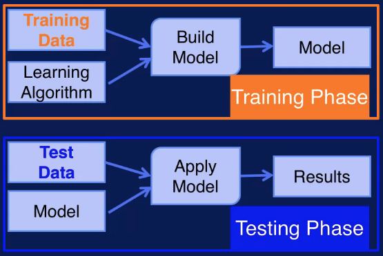
The error on the test data is an indication of how well the classifier will perform on new data. This is known as generalization. Generalization refers to how well your model performs on new data, that is data not used to train the model. You want your model to generalize well to new data. If your model generalizes well, then it will perform well on data sets that are similar in structure to the training data, but doesn't contain exactly the same samples as in the training set. Since the test error indicates how well your model generalizes to new data, note that the test error is also called generalization error.

A related concept to generalization is overfitting. If your model has very low training error but high generalization error, then it is overfitting. This means that the model has learned to model the noise in the training data, instead of learning the underlying structure of the data. The model tries to capture every sample point, instead of the general trend of the samples together.

The training error and the generalization error are plotted together, during model training. What is the connection between overfitting and generalization? A model that overfits will not generalize well to new data. So the model will do well on just the data it was trained on, but given a new data set, it will perform poorly.

A problem related to overfitting is underfitting. Overfitting occurs when the model is fitting to the noise in the training data. This results in low training error and high test error. Underfitting on the other hand, occurs when the model has not learned the structure of the data. This results in high training error and high test error.

Both are undesirable, since both mean that the model will not generalize well to new data. Overfitting generally occurs when a model is too complex, that is, it has too many parameters relative to the number of training samples. So to avoid overfitting, the model needs to be kept as simple as possible, and yet still solve the input/output mapping for the given data set.

Overfitting in Decision Trees

During the construction of a decision tree, also referred to as tree induction, the tree repeatedly splits the data in a node in order to get successively paired subsets of data. Note that a decision tree classifier can potentially expand its nodes until it can perfectly classify samples in the training data. But if the tree grows nodes to fit the noise in the training data, then it will not classify a new sample well. This is because the tree has partitioned the input space according to the noise in the data instead of to the true structure of a data. In other words, it has overfit.

How can overfitting be avoided in decision trees? There are two ways. One is to stop growing the tree before the tree is fully grown to perfectly fit the training data. This is referred to as pre-pruning. The other way to avoid overfitting in decision trees is to grow the tree to its maximum size and then prune the tree back by removing parts of the tree. This is referred to as post-pruning. In general, overfitting occurs because the model is too complex. For a decision tree model, model complexity is determined by the number of nodes in the tree. Addressing overfitting in decision trees means controlling the number of nodes. Both methods of pruning control the growth of the tree and consequently, the complexity of the resulting model.

With pre-pruning, the idea is to stop tree induction before a fully grown tree is built that perfectly fits the training data. To do this, restrictive stopping conditions for growing nodes must be used. For example, a node stops expanding if the number of samples in the node is less than some minimum threshold. Another example is to stop expanding a node if the improvement in the impurity measure falls below a certain threshold.

In post-pruning, the tree is grown to its maximum size, then the tree is pruned by removing nodes using a bottom up approach. That is, the tree is trimmed starting with the leaf nodes. The pruning is done by replacing a subtree with a leaf node if this improves the generalization error, or if there is no change to the generalization error with this replacement. In other words, if removing a subtree does not have a negative effect on the generalization error, then the nodes in that subtree only add to the complexity of the tree, and not to its overall performance. So those nodes should be removed. In practice, post-pruning tends to give better results. This is because pruning decisions are based on information from the full tree. Pre-pruning, on the other hand, may stop the tree growing process prematurely. However, post-pruning is more computationally expensive since the tree has to be expanded to its full size.

Using a Validation Set

A validation set can be used to guide the training process to avoid overfitting and deliver good generalization performance. We have discussed having a training set and a separate test set. The training set is used to build a model and the test set is used to see how the model performs a new data. Now we want to further divide up the training data into a training set and a validation set. The training set is used to train the model as before and the validation set is used to determine when to stop training the model to avoid overfitting, in order to get the best generalization performance.

The idea is to look at the errors on both training set and validation set during model training as shown here. The orange solid line on the plot is the training error and the green line is the validation error. We see that as model building progresses along the x-axis, the number of nodes increases. That is the complexity of the model increases. We can see that as the model complexity increases, the training error decreases. On the other hand, the validation error initially decreases but then starts to increase

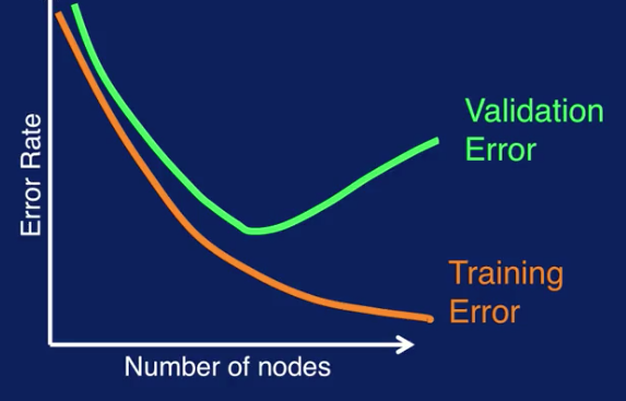
When the validation error increases, this indicates that the model is overfitting, resulting in decreased generalization performance.

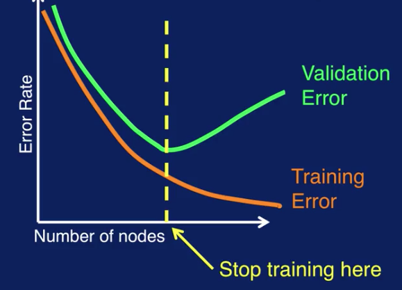
This can be used to determine when to stop training. Where validation error starts to increase is when you get the best generalization performance, so training should stop there. This method of using a validation set to determine when to stop training is referred to as model selection since you're selecting one from many of varying complexities. Note that this was illustrated for a decision tree classifier, but the same method can be applied to any type of machine learning model. There are several ways to create and use the validation set to avoid overfitting. The different methods are holdout method, random subsampling, k-fold cross-validation, and leave-one-out cross-validation.

Holdout

The first way to use a validation set is the holdout method. This describes the scenario that we have been discussing, where part of the training data is reserved as a validation set. The validation set is then the holdout set.

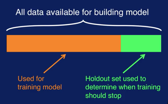
Errors on the training set and the holdout set are calculated at each step during model training and plotted together as we've seen before. And the lowest error on the holdout set is when training should stop. This is the just the process that we have described here before. There's some limitations to the holdout method however. First, since some samples are reserved for the holdout validation set, the training set now has less data than it originally started out with. Secondly, if the training and holdout sets do not have the same data distributions, then the results will be misleading. For example, if the training data has many more samples of one class and the holdout dataset has many more samples of another class.

The next method for using a validation set is repeated holdout. As the name implies, this is essentially repeating the holdout method several times. With each iteration, samples are randomly selected from the original training data to create the holdout validation set. This is repeated several times with different training and validation sets. Then the iterates on the holdout set for the different iterations are averaged together to get the overall iterate for model selection. A potential problem with repeated holdout is that you could end up with some samples being used more than others for training. Since a sample can be used for either testing or training any number of times, some samples may be put in the training set more times than other samples. So you might end up with some samples being overrepresented while other samples are underrepresented in training or testing. A way to improve on the repeated holdout method is use cross-validation.

K-Fold Cross-Validation

Cross-validation works as follows. Segment the data into k number of disjoint partitions. During each iteration, one partition is used as the validation set. Repeat the process k times. Each time using a different partition for validation. So each partition is used for validation exactly once.

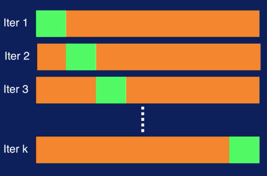
In the fist iteration, the first partition, specified in green, is used for validation. In the second iteration, the second partition is used for validation and so on. The overall validation error is calculated by averaging the validation errors for all k iterations. The model with the smallest average validation error then is selected. This approach gives you a more structured way to divide available data up between training and validation datasets and provides a way to overcome the variability in performance that you can get when using a single partitioning of the data.

Leave-one-out Cross-Validation

Leave-one-out cross-validation is a special case of k-fold cross-validation where k equals N, where N is the size of your dataset.

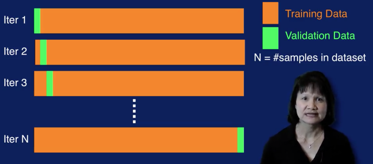
Here, for each iteration the validation set has exactly one sample. So the model is trained to using N minus one samples and is validated on the remaining sample. The rest of the process works the same way as regular k-fold cross-validation. Note that cross-validation is often abbreviated CV and leave-one-out cross-validation is in abbreviated L-O-O-C-V and pronounced LOOCV.

Datasets

Note that the validation error that comes out of this process can also be used to estimate generalization performance of the model. In other words, the error on the validation set provides an estimate of the error on the test set. With the addition of the validation set, you really need three distinct datasets when you build a model.

The training dataset is used to train the model, that is to adjust the parameters of the model to learn the input to output mapping.

The validation dataset is used to determine when training should stop in order to avoid overfitting.

The test data set is used to evaluate the performance of the model on new data. Note that the test data set should never, ever be used in any way to create or tune the model. It should not be used, for example, in a cross-validation process to determine when to stop training.

The test dataset must always remain independent from model training and remain untouched until the very end when all training has been completed. Note that in sampling the original dataset to create the training, validation, and test sets, all datasets must contain the same distribution of the target classes. For example, if in the original dataset, 70% of the samples belong to one class and 30% to the other class, then this same distribution should approximately be present in each of the training, validation, and test sets. Otherwise, analysis results will be misleading.

Metrics to Evaluate Model Performance

For the classification task, an error occurs when the model's prediction of the class label is different from the true class label. We can also define the different types of errors in classification depending on the predicted and true labels. Then the different types of errors are as follows.

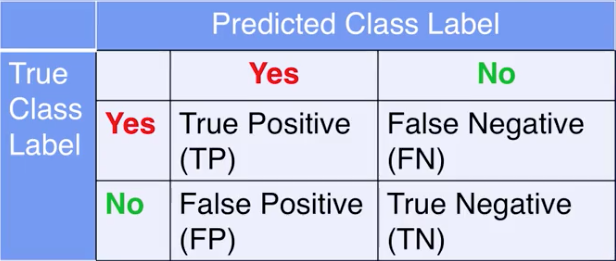
If the true label is yes and the predicted label is yes, then this is a true positive, abbreviated as TP. This is the case where the label is correctly predicted as positive.

If the true label is no and the predicted label is no, then this is a true negative, abbreviated as TN. This is the case where the label is correctly predicted as negative.

If the true label is no and the predicted label is yes, then this is a false positive, abbreviated as FP. This is the case with the label is incorrectly predicted as positive, when it should be negative.

If the true label is yes and the predicted label is no, then this is a false negative abbreviated as FN. This is the case where the label is incorrectly predicted as negative, when it should be positive.

Accuracy and Error Rate

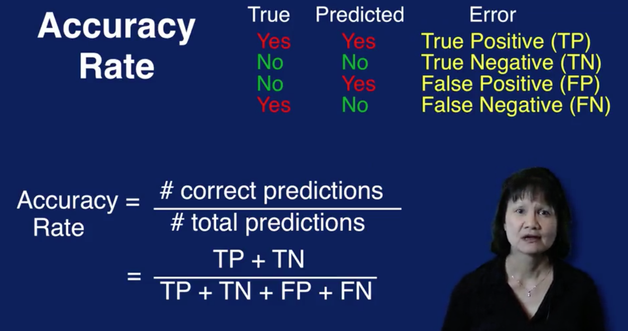
These four different types of errors are used in calculating many evaluation metrics for classifiers. The most commonly used evaluation metric is the accuracy rate, or accuracy for short. For classication, accuracy is calculated as the number of correct predictions divided by the total number of predictions.

Note that the number of correct predictions is the sum of the true positives, and the true negatives, since the true and predicted labels match for those cases. The accuracy rate is an intuitive way to measure the performance of a classification model.

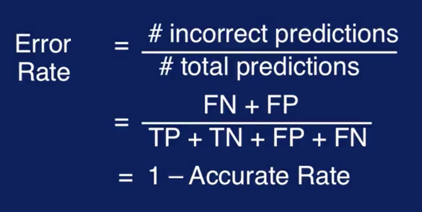
Model performance can also be expressed in terms of error rate. Error rate is the opposite of accuracy rate.

There's a limitation with accuracy and error rates when you have a class imbalance problem. This is when there are very few samples of the class of interest, and the majority are negative examples. An example of this is identifying if a tumor is cancerous or not. What is of interest is identifying samples with cancerous tumors, but these positive cases where the tumor is cancerous are very rare. So, you end up with a very small fraction of positive samples, and most of the samples are negative. Thus the name, class imbalance problem.

What could be the problem with using accuracy for a class imbalance problem? Consider the situation where only 3% of the cases are cancerous tumors. If the classification model always predicts non-cancer, it will have an accuracy rate of 97%, since 97% of the samples will have non-cancerous tumors. But note that in this case, the model fails to detect any cancer cases at all. So the accuracy rate is very misleading here. You may think that your model is performing very well with such a high accuracy rate. But in fact it cannot identify any of the cases in the class of interest. In these cases we need evaluation metrics that can capture how well the model classifies positive, versus negative classes.

Precision and Recall

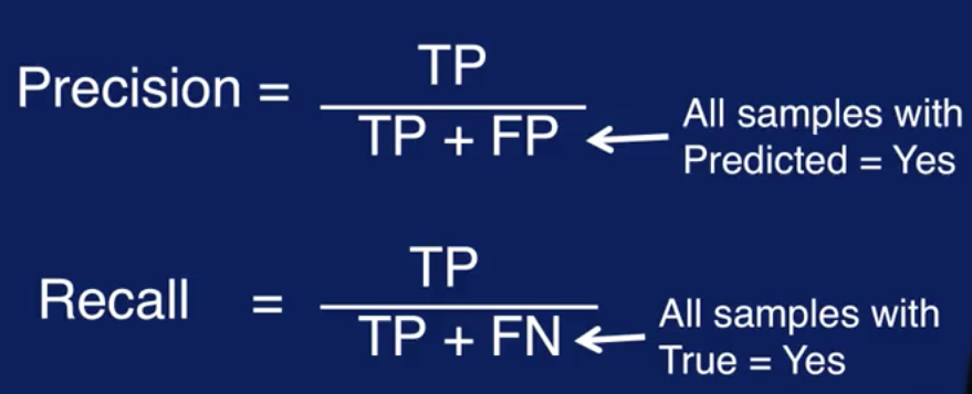
A pair of evaluations metrics that are commonly used when there is a class imbalance are precision and recall. Precision is defined as the number of true positives divided by the sum of true positives and false positives. In other words, it is the number of true positives divided by the total number of samples predicted as being positive. Recall is defined as the number of true positives divided by the sum of true positives and false negatives. It is the number of true positives divided by the total number of samples, actually belonging to the true class

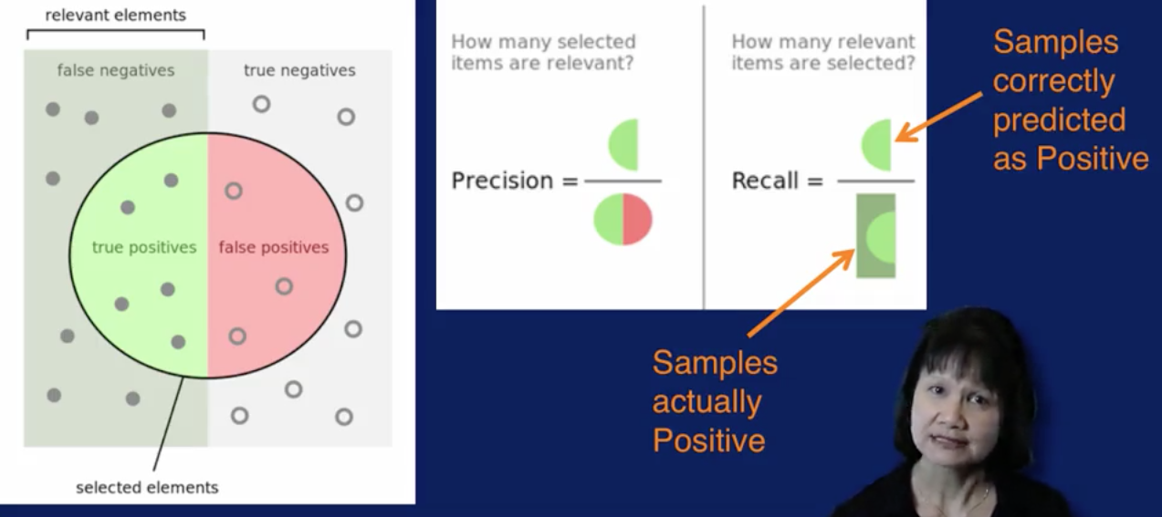
The selected elements indicated by the green half circle are the true positives. That is samples predicted as positive and are actually positive. The relevant elements indicated by the green half circle and the green half rectangle, are the true positives, plus the false negatives. That is samples that are actually positive, but some are correctly predicted as positive, and some are incorrectly predicted as negative. Recall then is the number of samples correctly predicted as positive, divided by all samples that are actually positive.

The entire circle indicated by the green half circle and the pink half circle, are the true positives plus the false positives. That is samples that were predicted as positive although some were actually positive and some were actually negative. Then precision is the number of samples correctly predicted as positive, divided by the number of all samples predicted as positive.

Precision is considered a measure of exactness because it calculates the percentage of samples predicted as positive, which are actually in a positive class. Recall is considered a measure of completeness, because it calculates the percentage of positive samples that the model correctly identified.

There is a trade off between precision and recall. A perfect precision score of one for a class C means that every sample predicted as belonging to class C, does indeed belong to class C. But this says nothing about the number of samples from class C that were predicted incorrectly. A perfect recall score of one for a class C, means that every sample from class C was correctly labeled. But this doesn't say anything about how many other samples were incorrectly labeled as belonging to class C. So they are used together. The goal for classification is to maximize both precision and recall.

F-Measure

Precision and recall can be combined into a single metric called the F-measure. The equation for that is 2 times the product of precision and recall divided by their sum. There are different versions of the F-measure.

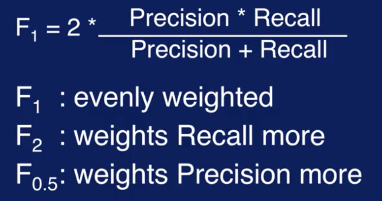
The value for the F1 measure ranges from zero to one, with higher values giving better classification performance.

Confusion Matrix

A Confusion Matrix can be used to summarize the different types of classification errors. Each cell has the count, or percentage of samples, with each type of errors.

The higher the sum of the diagonal values, the better the performance of the model. The off diagonal values capture the misclassified samples. Where the model's predictions do not match the true labels.

The sum of the diagonal values in a confusion matrix, divided by the total number of samples gives you the Accuracy Rate. Similarly, the off diagonal values are related to the Error Rate. The sum of the off diagonal values in a confusion matrix, divided by the total number of samples, gives you the Error Rate.

Looking at the values in the Confusion Matrix can help you understand the kind of Misclassifications that your model is making. A high value in the FN cell means that classifying the Positive class is problematic for the model. A high value for the cell FP on the other hand, means that classifying the Negative class is problematic for the model.